The Smithsonian Open Access release has put a trove of cultural heritage digital assets and data in the public commons. I wanted to show how you could start exploring and using the data. If you are comfortable running some Python scripts this post will quickly give you a head start. If not you might still be interested in following along as we look at some discoveries and visualizations I’ve created along the way.

The first step is to get the data. The site details there is an API and also a Github repository. We want to work with all the data so we are going straight for the Github. While the nearly 3 million digital items are the stars of the show there is in total over 11 million records in this data release. The repository is structured with each division having its own directory with many metadata files in each compressed as bz2 archives. These BZIP2 files are similar to the ubiquitous ZIP file but offer better compression ratios. Let’s download the data, we are going to be using MacOS or Linux command line:

	curl -L https://github.com/Smithsonian/OpenAccess/archive/master.zip --output data.zip
	unzip data.zip

We now want to now get at the metadata in the bz2 files. We are going to use this python script to traverse all the files, extract the data and write it to one large newline delimited JSON file. Once all the records are compiled into one file, with one record per line, it will be much quicker to iterate over all 11M records.

	import glob
	import bz2

	with open('all_data.ndjson','w') as out:
	  for div in glob.glob('./OpenAccess-master/metadata/objects/*'):
	    print('Working on: ',div)
	    for file in glob.glob(f'{div}/*'):
	      with bz2.open(file, "rb") as f:
	        out.write(f.read().decode())

The code used for this project can be found here

You will want to have 26GB of free space to run this script.

We now have all the data extracted and we can start exploring. 11 million records is a lot, for real, but we can still work with it using a single python script in this format, one line at a time. We will use one advantage however, we are going to install and use the UltraJSON python module to do our JSON interactions. This module is much faster at decoding JSON strings than the JSON module that comes with Python. So make sure to install it using the pip3 install ujson command.

The first step is to figure out what fields we have available to us. Each record a content field that contains three top level elements: descriptiveNonRepeating, indexedStructured and freetext. These are pretty self-describing but it looks like (I have no inside knowledge, this is the first time I’m seeing this data, so I’m making a lot of assumptions) that descriptiveNonRepeating is the basic data present on all records, things like what department it came from. indexedStructured is data that has been somewhat normalized already and is fairly common across all records, like date. And freetext which is more domain specific and or non-normalizable, things like note fields.

One important field in the descriptiveNonRepeating data is online_media which seems to tell us where to find the digital asset. Out of the 11M records not all of them have digital components. Here are two charts showing which divisions have what percentage of the digital assets, and what percentage of records with no digital items:

These charts show us a number of things including that right now the vast majority of records with media links are from the NMNH Botany Department.

I also made a chart of what percentage of indexedStructured and freetext fields are available across all 11M records:

It looks like there is a lot of good data in indexedStructured for us to play around with. I’m assuming this data has been “cleaned up” and normalized making things a little more consistent. The first field we can look at is the date, looks like this field is related to the creation of the object and is rounded to the nearest decade:

Next let's look at the topic field, seems like these are subject heading type tags relating to the object. I pulled out all the topics by the department of the object. Click the name of the dept on the left to view the counts. These are the topics for 9.7M records.

I was going to map the geographic information for the 9.8M records that had the field. But it looked like there would be a lot of work geocode all the various labels to coordinates. So please just enjoy the JSON dump of the values instead (and feel free to map them!)

The data for these graphs was generated with this script.

The last thing I wanted to try was something with the freetext fields. These fields are not structured and nicely normalized as the previous fields. I wanted to try and plot all the dimensions of the objects to see the variation in the sizes. There was a physicalDescription field for 5.8M records. I used a few simple regular expressions to see if I could pull out centimeter measurements of the object where there was at least a height and width provided. This resulted in about 640K measurements that I plotted onto one image:

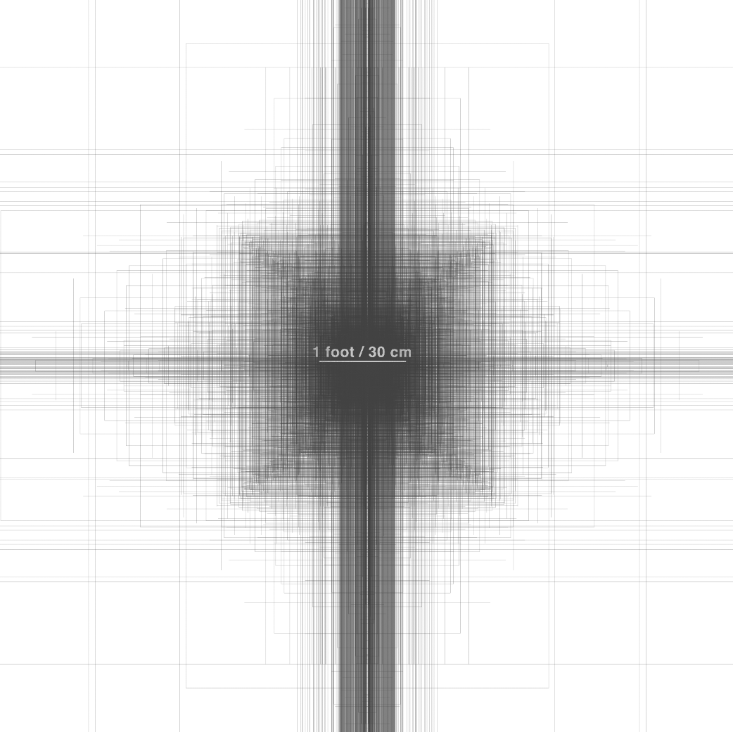
The entire image is about 24x24 feet. (Click to see the full resolution, 25K x 25K pixel image, but it might break your browser, be careful.) This script created the image.

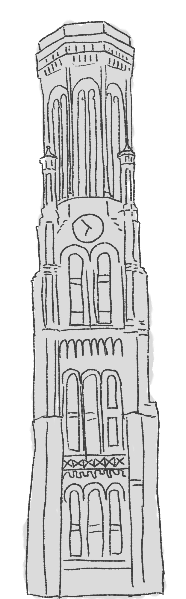
You can see most of the objects were less than one foot in height and width. Some of the strange outliers, like the very skinny and super tall outlines can be attributed to metadata quirks. Like this reportedly almost one mile (63,125 inches) tall pitcher. Metadata is hard and can go wrong in such suprising ways through migrations, transformations and maintenance, especially for 11M records.

We quickly looked at what you can do with just a few of these fields. But of course this barely scratches the surface of the possibilities. It also is only using the metadata, we haven’t even talked about the 3M digital items yet. This open access release is really a tremendous feat and credit to all who made it possible.